We assess the sensitivity of the NIPI's forecasting performance to two key parameters: the averaging window $\omega$ and the observation cutoff $\lambda$ . Through a grid search across six countries, we find that $\omega$ acts primarily as a noise filter while $\lambda$ is the active forecasting lever, with optimal values which will differ from one economy to the other.
Our language models detect news relevant to the near-term inflation forecast, then aggregate the signals in several ways. In recent notes we explored the extend to which our main diffusion index, the NIPI (News Inflationary Pressures Index), can lead official CPI releases. Here, we explore how inflation forecasts could be further optimized by tweaking some of the key parameters used to aggregate information in the NIPI.
A primer on the NIPI
Everyday, thousands of inflation related news are gathered by our language models. For a given country and a given sector, we quantify the sum of the probabilities of those news being positive to the near-term inflation outlook using specially trained language models (same goes for negative news).
The models assign a probability for each individual news to be positive or negative to the near-term inflation outlook. We then aggregate this information into two daily measures : $entr^{+}_{t}$ and $entr^{-}_{t}$, which are respectively the sum of the probabilities of news being positive and the sum of probabilities of news being negative. Both are accessible through API queries per direct CSV file download.
We then calculate the balance of positive and negative news, normalized into a diffusion index centered around 50 (to simplify the reading, so 50 = neutral like a PMI or ISM):
$$NIPI^{*}_{i} = (((entr^{+}_{t} \,–\, entr^{-}_{t}) / S ) +1 ) * 50$$
Note : S is sector and country-specific constant1.
That would be for a single day. Our reference metric, the NIPI, is the simple average of the last $\omega$ observations of $NIPI^{*}_{i}$. In the baseline specification, $\omega$ is set to 30.
The reading is meant to be straightforward : a NIPI value of 50 is indicative of a balanced volume of positive and negative inflation news, a value above 50 indicates positive inflationary pressures in the near-term and vice-versa.
Chart 1 : NIPI overview
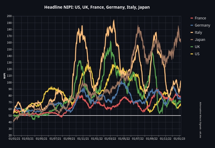
Chart 1 shows the NIPI across a range of countries and illustrates common cycles and desyncronization phases. While the NIPI series share common swings, their amplitude, persistence and timing differ. This raises a logical question: does the baseline configuration equally fit economies of various size and cycle?
Fine tuning the NIPI for forecasting
Data overview
We check how the NIPI parameters help improve or not the diffusion index’s ability to forecast near-term inflation. The target variables are Consumer Price Indices in the United States, France, Germany, Italy, the United Kingdom and Japan (more precisely, the HICP in European countries). The following table summarizes where the data come from and which transformations are applied.
Table 1 : CPI and HICP’ sources and transformations.
| Country | Source | Seasonal Adjustment | Release date* |
|---|---|---|---|
| US | Bureau of Labour Statistics | Provided Seasonally Adjusted | 42 days |
| France | Eurostat | Obtained using X13 ARIMA-SEATS | 30 days |
| Germany | Eurostat | Obtained using X13 ARIMA-SEATS | 28 days |
| Italy | Eurostat | Obtained using X13 ARIMA-SEATS | 30 days |
| UK | Office for National Statistics | Obtained using X13 ARIMA-SEATS | 47 days |
| Japan | Japanese Statistics Bureau | Provided Seasonally Adjusted | 51 days |
| * from 1st day of the month, on average |
The seasonally-adjusted series2 are used to compute month-on-month growth rates. Each CPI observation is dated to its actual publication day rather than its reference month. This ensures that the NIPI entering the model only reflects news available before the print is released.
We use NIPI Headlines from each of the 6 countries. Seasonality is not found to be statistically evident in the Headline NIPI series, so no further adjustment is made. The NIPI metrics are de facto stationary (hovering around 50), so they should enter inflation models in level.
Model specification
We use a simple AR(1) model augmented by a NIPI term to forecast Seasonally adjusted CPIs MoM%, yielding this specification :
$$\pi_{i,t} = \alpha_i + \gamma_i \pi_{i,t-1} + \beta_i \, NIPI^{\omega}_{i,t-\lambda} + \varepsilon_{i,t}$$
Each country $i$ is estimated independently.
Optimization framework
In another note we found that the optimal lag, i.e. the NIPI cutoff before the CPI print, was key yet disparate, even within a sample limited to European economies.
Here we add the window length $\omega$ to the optimization, testing whether a shorter or longer rolling period could better suit some countries in a forecasting context.
The interactive widget below illustrates the two parameters at play: $\omega$ controls the length of the averaging window, while $\lambda$ sets how many days before the CPI publication we stop reading news. Together, they determine which slice of daily entropy data feeds into the NIPI used for forecasting.
We evaluate the different NIPI configurations performances, depending both on the window length $\omega$ and on the cutoff $\lambda$. The out-of-sample forecasts are run from January 2020 to March 2026, covering a complete inflation cycle and facing the 2021/2022 crisis with no look-ahead bias: at each step, the model is estimated using only data available at the time of the forecast.
Results
The following heatmaps demonstrate how each specification scores against an AR(1) process depending on the two parameters. Both parameters are tested over a grid ranging from 5 to 90 days with a one-day step, yielding over 7000 combinations per country.
A first group of countries made of France, Germany, Italy and Japan displays a stable performance surface across most of the parameter space. For these economies, the NIPI beats the AR(1) benchmark under a wide range of ($\lambda$, $\omega$) combinations, and the optimal specification offers only marginal gains over the baseline.
Chart 2: Heat-map performances : Germany
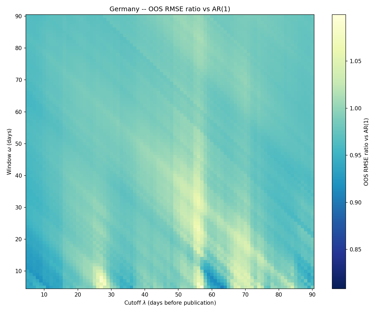
Chart 3: Heat-map performances : France
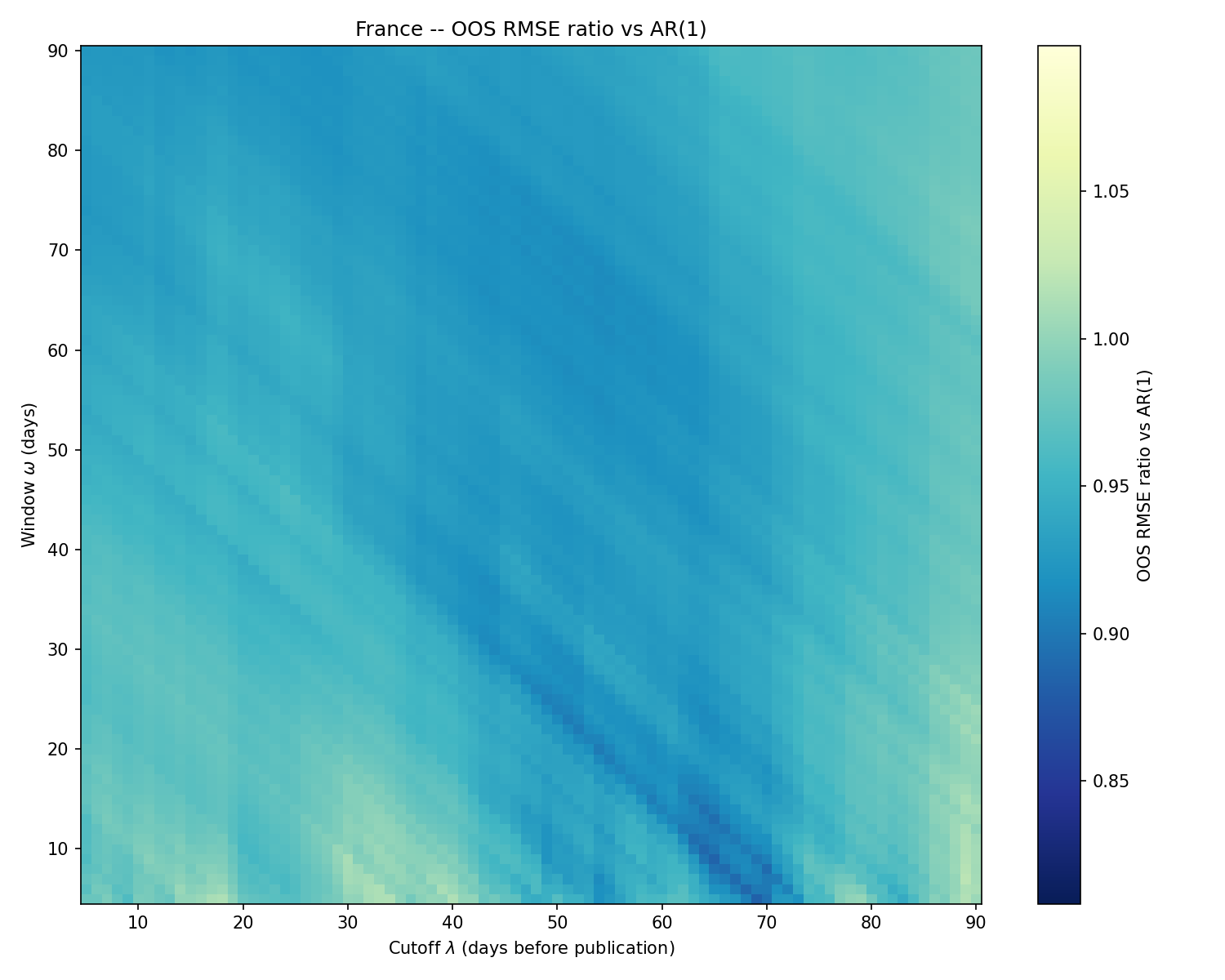
Chart 4: Heat-map performances : Italy
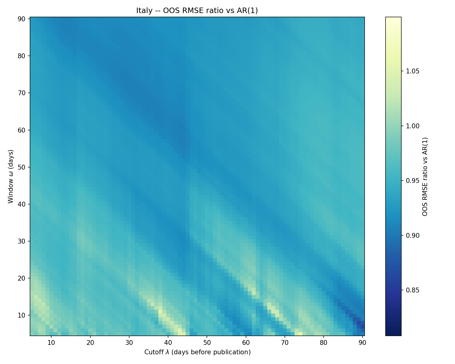
Chart 5: Heat-map performances : Japan
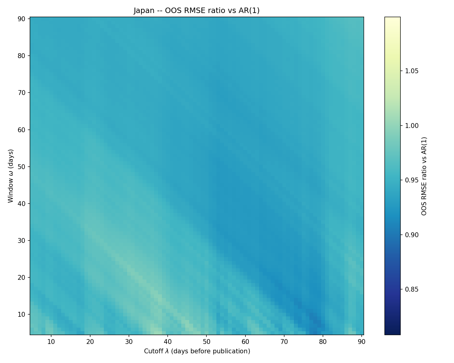
The only notable pattern is the instability visible in the lower region of the heatmaps, where $\omega$ falls below 15-20 days. With fewer observations in the averaging window, the signal becomes too noisy to provide stable forecasting gains. Beyond that threshold, neither $\omega$ nor $\lambda$ meaningfully discriminates across specifications.
The baseline NIPI ($\omega$ = 30) already sits comfortably in the stable region, and no country-specific tuning is warranted. This robustness does not hold universally, however. A different picture emerges for the United States and the United Kingdom, where the choice of parameters has a markedly stronger impact on the forecasting performance.
Chart 6: Heat-map performances : United States
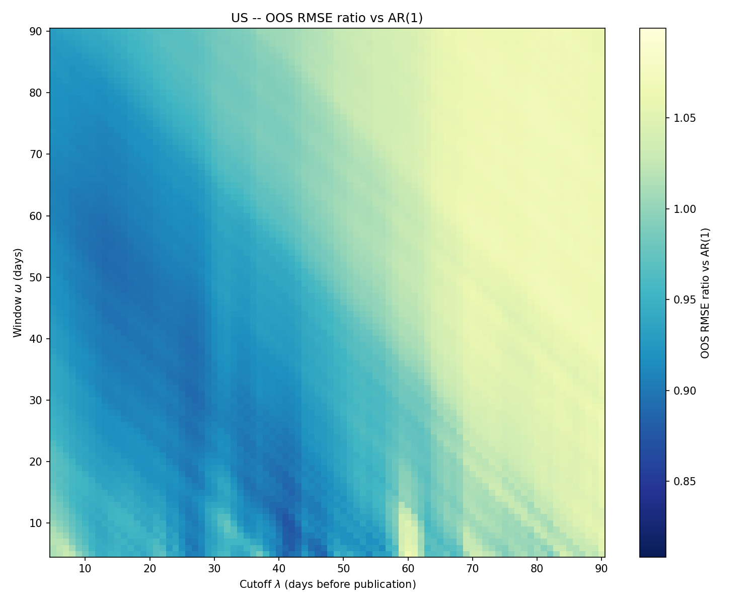
Chart 7: Heat-map performances : United Kingdom
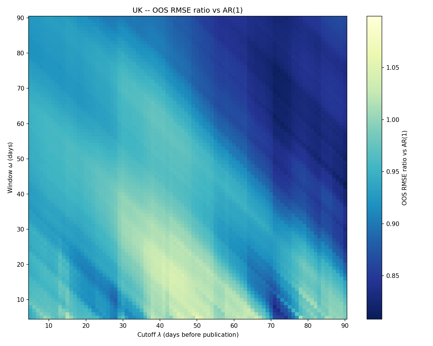
Both heatmaps exhibit clear directional trends but also localized noise, particularly at low omega. To identify the most robust specification rather than an isolated optimum, we smooth the performance surface using a median filter (11-day radius) and select the point minimizing the filtered ratio.
Chart 8: Smoothed heat-map performances : United States
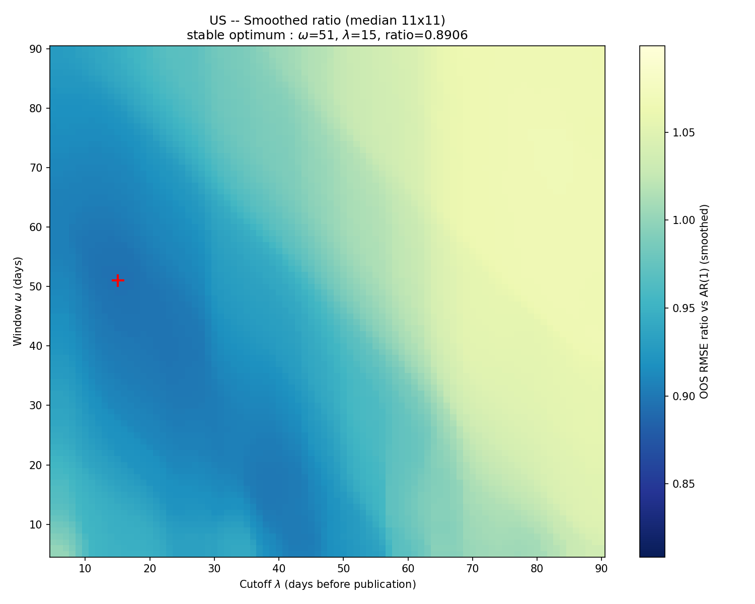
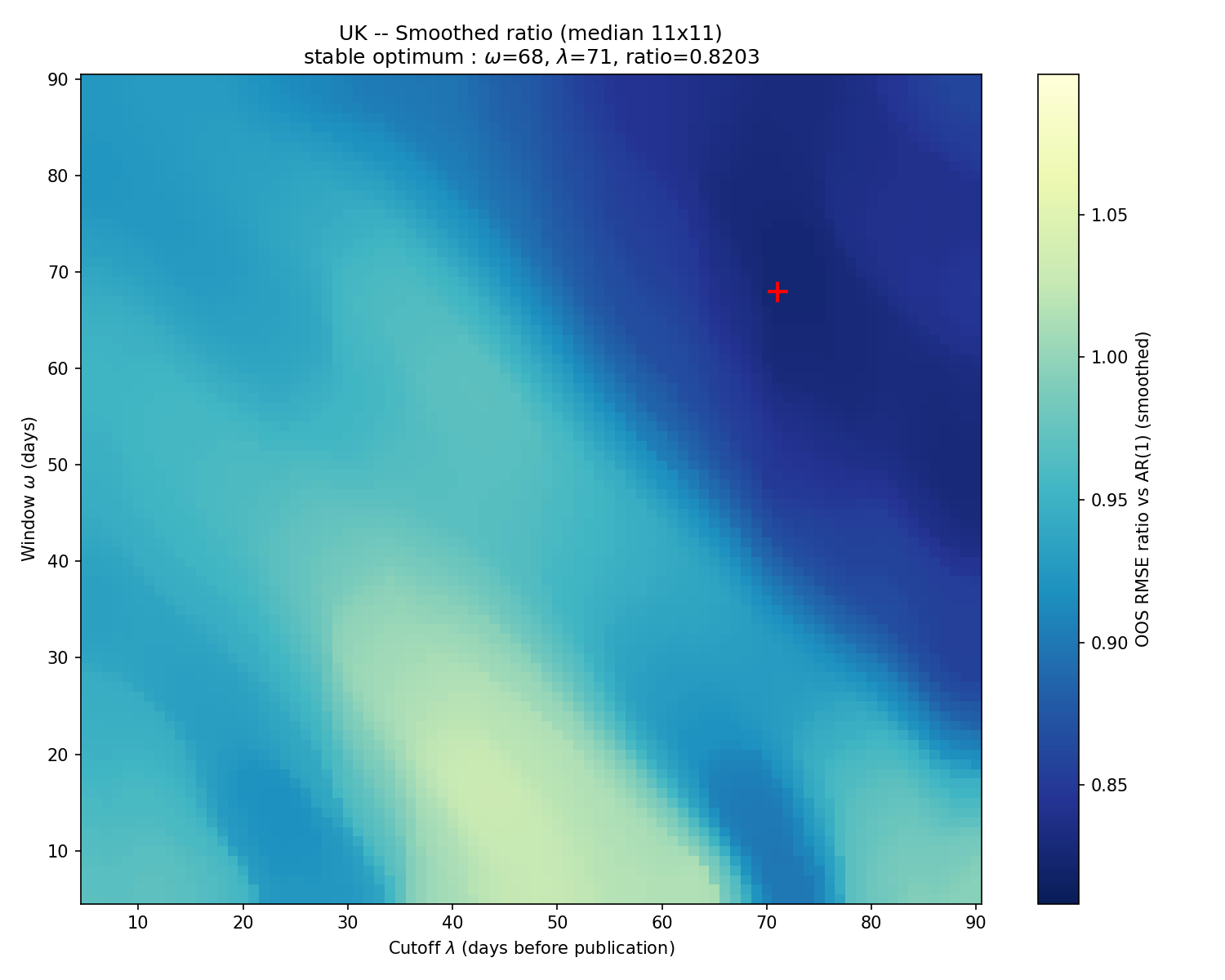
Chart 9: Smoothed heat-map performances : United Kingdom
Regarding the United States, the stable optimum concentrates around a short cutoff (lambda around 15 days) and a slightly larger than usual window (omega around 50 days). The signal is most informative when sampled close to the publication date, consistent with the fast transmission of inflation news in the US economy (and a late typical CPI release date, when compared with Europe).
Concerning the United Kingdom, the optimal combination would imply much higher parameter values : the smoothed head-maps suggest the optimal ambda hovers around 70 and optimal omega around 70. The UK NIPI requires a longer lookback and an earlier cutoff to be informative, suggesting a slower transmission from news to prices.
These varying optimal specifications reflect distinct price formation mechanisms across economies. Inflation news does not feed into prices at the same speed everywhere, and the forecasting framework should account for this heterogeneity rather than impose a universal specification.
Based on the stable-performance regions identified above, the following table suggests a practical specification for each country. It shows the recommended parameters applied to the next CPI release as an exemple and report the implied entropy window feeding into the NIPI.
Table 2 : Recommended specification and application
| Country | $\lambda$ | $\omega$ | Upcoming CPI prints | Implied Entropy Window |
|---|---|---|---|---|
| US | 15 | 50 | 10th June 2026 (May) | Apr 7th to May 26th |
| France | 30 | 30 | 30th May 2026 (June) | May 2nd to May 31st |
| Germany | 30 | 30 | 29th May 2026 (June) | May 1st to May 30th |
| Italy | 30 | 30 | 30th May 2026 (June) | May 2nd to May 31st |
| UK | 70 | 70 | 17th June 2026 (May) | Jan 29th to Apr 8th |
| Japan | 30 | 30 | 19th June 2026 (May) | Apr 21th to May 20th |
The first group of countries shows no meaningful gain from tuning: $\omega$ = 30 and $\lambda$ = 30 are retained as conservative defaults, consistent with the flat performance surface observed above. The United States and United Kingdom are assigned the stable optima identified through the median-filtered surface.
Summing up our main findings
- The NIPI beats the AR(1) benchmark across all six countries, confirming its value as a forecasting input regardless of the specification chosen.
- Neither parameter discriminates for most economies; where it matters (US, UK), the cutoff $\lambda$ is the active lever.
- The window length $\omega$ acts primarily as a noise filter and should be set to a conservative floor.
The daily granularity of the underlying signal is what makes this analysis possible in the first place: with a monthly indicator, neither the cutoff nor the window could be calibrated at this resolution. As the dataset expands, further dimensions could be explored, such as sector-level disaggregation or the inclusion of the neutral Entropy metric in the NIPI construction.
↩ 1 S is defined as the maximum between Q and 3. Q being the 0.90 quantile value of the total number of news (relevant news, whatever their sign) series range over the period 2018-2020 for the corresponding country and sector.
↩ 2 Accounting for trading days and country-specific public holidays, for each country, we isolate the seasonal components from CPI.
To know more about our data,reach out.
