The News Inflationary Pressures Indices (NIPI) are built to capture hard-to-catch macroeconomic information from “events” or “news” with an expected imminent impact on inflation. But do they really convey information above and beyond usual time series? In this note, we show that when a NIPI-only short-term inflation model is augmented by weekly petrol prices in Europe, there is no information redundancy: the NIPI information content is preserved and we do observe a broad-based improvement in out-of-sample forecast accuracy. In short: there is a lot more to the NIPI than petrol prices.
In our data, we retrieve macroeconomic signals from text data only – using specially trained language models out-of-sample.
In earlier blog posts, we have illustrated the extent to which the NIPI can help forecast near-term inflation developments in the US, Europe or at the global level on its own . There is, indeed, strong statistical evidence that systematic news processing is relevant to near-term inflation forecasting and provides timely information for short-term monitoring. The NIPI is available daily with almost no lag, which is a tremendous advantage to forecasting near-term inflation.
But how unique is the kind of information contained in the NIPI ? While the NIPI can help identify information that does not fit in time series (for instance changes in excise duties or product shortages), precisely what the models have been built for, it is also fair to say the NIPI likely contains information which could be available in time series, to some degree.
Petrol prices are the perfect test. The NIPI does capture petrol price changes, large changes at least, which usually feature prominently in the news headlines. In countries where petrol prices are available at weekly (in Europe) or daily (US) frequency, such information is somewhat redundant, and if the NIPI could not add to it, it would simply be useless.
The bar to add information is actually higher than it seems: many high-frequency inflation indicators actually struggle to add significant information to daily petrol prices.
So we have built an experiment to test the extent to which the NIPI information content is preserved when petrol price time series are incorporated.
Base model
Our starting point is a pooled panel model for nowcasting monthly CPI inflation across 9 European economies (France, Germany, Italy, Spain, Austria, Ireland, the Euro Area aggregate, the United Kingdom and Switzerland), which we presented in a previous note.
The model relies on two explanatory variables: a country-specific NIPI (14 calendar days before the start of the target month), and the first principal component of a broad CPI or HICP panel covering Euro Area member states, the United Kingdom and Switzerland (23 countries).
$$\pi_{i,t} = \alpha + \beta_i \, NIPI_{i,t-\lambda} + \gamma \, PC1_{t-1} + \varepsilon_{i,t}$$
The model is estimated by pooled OLS across all countries and validated on out-of-sample data using an expanding-window walk-forward exercise. It delivered an average RMSE improvement of 12% over a naive AR(1) benchmark.
This specification will be referred to as “V1” from now on.
Adding petrol
The European Commission publishes the Weekly Oil Bulletin, a dataset of retail fuel prices updated every Monday. We extract the Diesel and the SP95 (Euro-super 95) series, which serve as a high-frequency proxy for the retail energy component of HICP.
For each month, we retain the third-to-last weekly observation, which lies around the middle of the month and is available about two weeks before the HICP release. We then compute the month-on-month percentage change of SP95 and diesel prices and take their average.
$$\Delta petrol_{i,t} = \frac{1}{2}\left[\left(\frac{SP95_{i,t}}{SP95_{i,t-1}} - 1\right)\times 100 + \left(\frac{Diesel_{i,t}}{Diesel_{i,t-1}} - 1\right)\times 100\right]$$
Petrol interaction terms are included for the 7 entities covered by the Oil Bulletin: France, Germany, Italy, Spain, Austria, Ireland and the Euro Area aggregate.
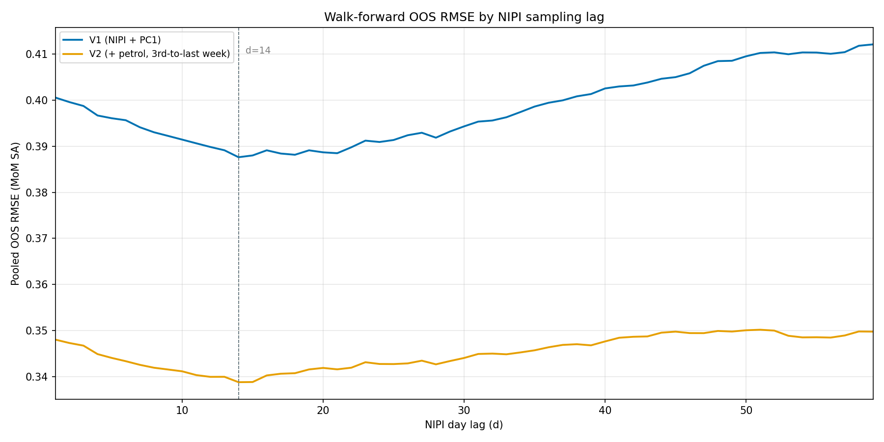
In the V1 specification, $\lambda$, i.e. the number of days before the start of the following month at which the NIPI is read, was set at 14 to maximize forecast accuracy. A grid-search on the augmented model confirms that this value remains appropriate: it preserves consistency with the original specification, aligns with the economic intuition behind the NIPI sampling window, and comes at no cost in terms of out-of-sample performance.
Chart 1: Model RMSE depending on $\lambda$
Results
The augmented model (V2) differs from the baseline (V1) only by the inclusion of the petrol prices terms. Both specifications are first estimated on the full sample, then evaluated through the same expanding-window walk-forward procedure, from January 2020 to August 2026, with about 80 out-of-sample observations per country.
On the full sample (Table 1), all NIPI coefficients remain positive and significant under V2. The petrol coefficients are positive and strongly significant for 6 of the 7 entities covered, Italy being the exception.
- Table 1: Loadings on the largest and latest estimation sample (2018-01 to 2026-08)
| Variable | V1 Coefficient | V2 Coefficient | V1 P-value | V2 P-value |
|---|---|---|---|---|
| $\alpha$ | -0.315 | -0.359 | <0.01 | <0.01 |
| ${NIPI}_{France, t-\lambda}$ | 0.0094 | 0.0099 | <0.01 | <0.01 |
| ${NIPI}_{Germany, t-\lambda}$ | 0.0097 | 0.0100 | <0.01 | <0.01 |
| ${NIPI}_{Italy, t-\lambda}$ | 0.0067 | 0.0073 | <0.01 | <0.01 |
| ${NIPI}_{Spain, t-\lambda}$ | 0.0104 | 0.0107 | <0.01 | <0.01 |
| ${NIPI}_{Austria, t-\lambda}$ | 0.0115 | 0.0121 | <0.01 | <0.01 |
| ${NIPI}_{Ireland, t-\lambda}$ | 0.0092 | 0.0104 | <0.01 | <0.01 |
| ${NIPI}_{Euro Area, t-\lambda}$ | 0.0107 | 0.0096 | <0.01 | <0.01 |
| ${PC1}_{t-1}$ | 0.0224 | 0.0183 | <0.01 | <0.01 |
| $\Delta{petrol}_{France, t}$ | 0.0326 | <0.01 | ||
| $\Delta{petrol}_{Germany, t}$ | 0.0449 | <0.01 | ||
| $\Delta{petrol}_{Italy, t}$ | 0.0034 | 0.70 | ||
| $\Delta{petrol}_{Spain, t}$ | 0.0381 | 0.02 | ||
| $\Delta{petrol}_{Austria, t}$ | 0.0396 | <0.01 | ||
| $\Delta{petrol}_{Ireland, t}$ | 0.0375 | <0.01 | ||
| $\Delta{petrol}_{Euro Area, t}$ | 0.0343 | <0.01 |
To assess forecasting performance, we turn to the expanding-window walk-forward exercise, in which the model is re-estimated each month on the data available up to that point. Across these re-estimations, the average in-sample R-squared rises from 0.267 (V1) to 0.465 (V2). Out of sample, the pooled m-o-m SA RMSE falls from 0.388 to 0.346, an 11% improvement.
Table 2: Expanding Out of Sample m-o-m% SA RMSE
| Country | V1 RMSE | V2 RMSE | Diff |
|---|---|---|---|
| France | 0.283 | 0.218 | -23% |
| Germany | 0.447 | 0.355 | -21% |
| Italy | 0.433 | 0.439 | +1% |
| Spain | 0.436 | 0.389 | -11% |
| Austria | 0.423 | 0.343 | -19% |
| Ireland | 0.370 | 0.347 | -6% |
| Euro Area | 0.282 | 0.218 | -23% |
Table 2 shows that the gains are broad-based but heterogeneous across countries. They are largest where the petrol loadings are significant (France, Germany, Austria and the euro area), while Italy is essentially unchanged, consistent with its insignificant petrol coefficient.
We then convert the m-o-m forecasts into y-o-y figures, first in SA terms, then in NSA terms by reapplying the seasonal factors available at the time of the forecast. The NSA figures allow both versions to be benchmarked against the market consensus.
Table 3: Expanding Out of Sample y-o-y% forecasting performance
| Country | V1 RMSE SA1 |
V2 RMSE SA |
V1 RMSE NSA1 |
V2 RMSE NSA |
Consensus RMSE NSA |
N2 | DM test3 V2 SA / Consensus | DM test V2 NSA / Consensus |
|---|---|---|---|---|---|---|---|---|
| France | 0.291 | 0.213 | 0.400 | 0.331 | 0.269 | 67 | -2.16** | +2.34** |
| Germany | 0.471 | 0.372 | 0.596 | 0.465 | 0.364 | 80 | 0.17 | +1.80* |
| Italy | 0.471 | 0.478 | 0.622 | 0.631 | 0.496 | 74 | -0.54 | +2.97*** |
| Spain | 0.463 | 0.415 | 0.611 | 0.541 | 0.483 | 76 | -1.44 | +1.42 |
| Euro Area | 0.295 | 0.227 | 0.355 | 0.28 | 0.224 | 80 | 0.12 | +1.76* |
Over the January 2020 to August 2026 period, V2 outperforms V1 in every country except Italy, where the fuel price variable is not significant (our take is that Italy would probably warrant a slightly different petrol price specification than the general formulation). As expected, these gains mirror those on month-on-month SA figures, since the year-on-year error is driven by the target month alone.
Moving from SA to NSA figures mechanically increases the RMSE, as seasonal adjustment errors add to the model error, raising the V2 RMSE by 23% (euro area) to 55% (France). These errors are common to both specifications and lie outside the scope of the model.
On published (NSA) figures, the consensus remains more accurate than V2, significantly at the 5% level for France and Italy and at the 10% level for Germany and the euro area, with no significant difference for Spain. The error attributable to the model alone (SA columns) is, however, significantly lower than the consensus error for France, lower but not significantly so for Spain and Italy, and statistically indistinguishable for Germany and the euro area. The gap on NSA figures therefore stems mainly from the reseasonalization step, which constitutes the main lever for improvement.
Beyond accuracy, timeliness matters. Chart 2 tracks the out-of-sample RMSE of the model on y-o-y SA figures, day by day, from 45 days before the HICP flash release to the eve of the release.
Chart 2: Accuracy path of the two models
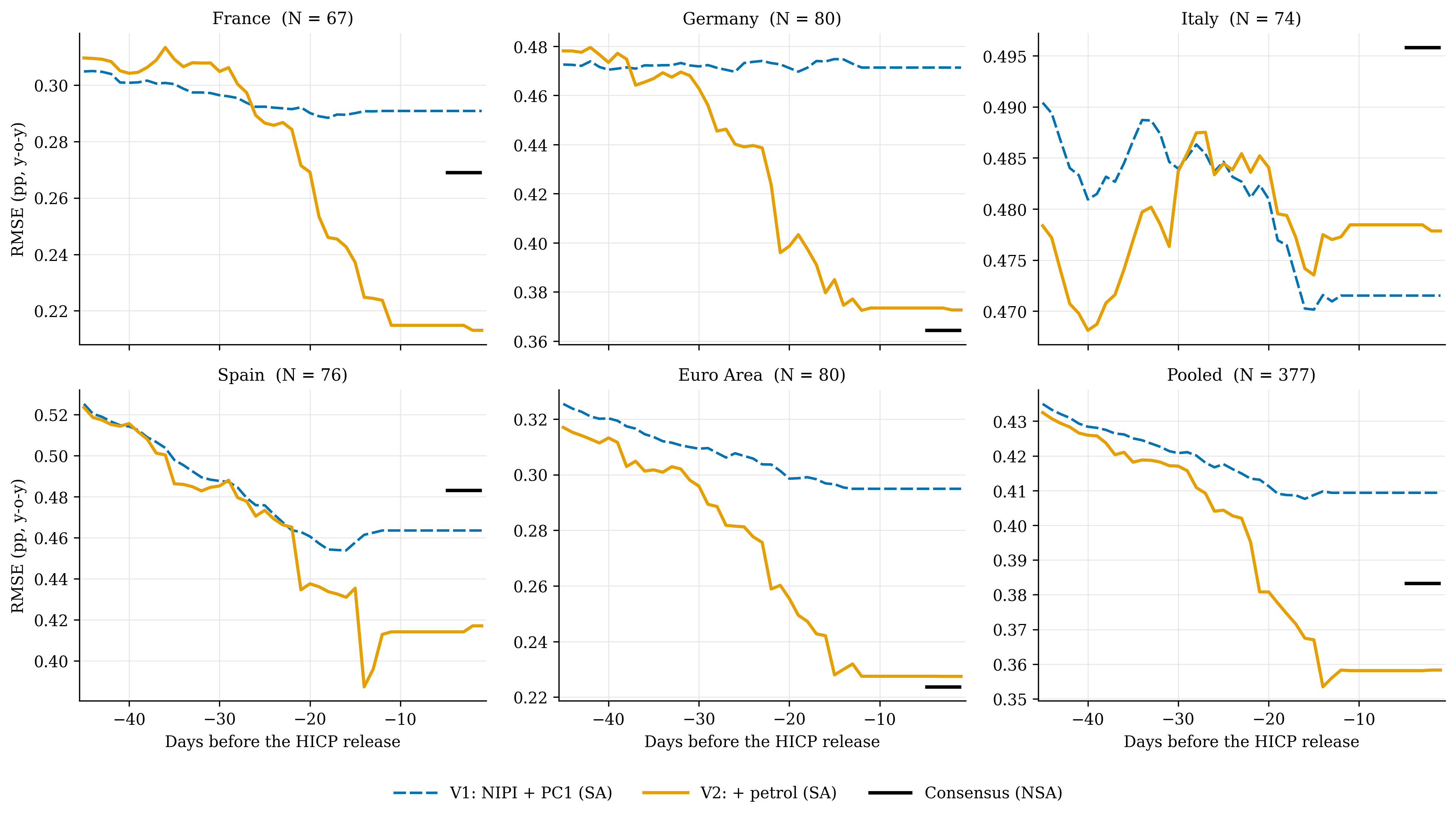
V2 improves steadily as weekly Oil Bulletin prices are published, and its forecast is final about two weeks before the release, once the third-to-last weekly price of the month is available. The consensus, where available, is only compiled in the last days before the release: it is shown as a fixed level over the final five days, evaluated on published NSA figures. The model thus delivers its final forecast around ten days before the consensus.
This note extends the NIPI-based European inflation nowcasting model by incorporating a direct measure of retail energy price dynamics.
We show that the NIPI does contain significant information beyond petrol prices and that a model combining the two data sources has convincing forecast ability.
In most cases, the forecast model can perform at least as well as consensus, while being available around 10 days earlier than consensus.
Going forward, we will deploy this augmented specification ahead of each HICP release to assess whether the level suggested by our NIPI-based model deviates meaningfully from the market consensus. Persistent or large gaps between the model and expectations will serve as an early signal of potential surprises in the official print.
↩ 1 SA: y-o-y changes of the seasonally adjusted series. NSA: y-o-y changes of the published, non seasonally adjusted series, obtained by reapplying real-time seasonal factors to the model forecasts.
↩ 2 Number of months between January 2020 and August 2026 for which both model and consensus forecasts are available.
↩ 3 Two-sided Diebold-Mariano test. Positive values favour the Consensus. *** p < 0.01, ** p < 0.05, * p < 0.10.
To know more about our data,reach out.
